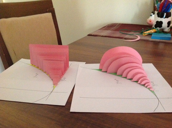
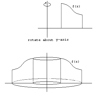
This week we focused on cross sections. Cross sections are three dimensional shapes whose length and width are determined by two functions, and depths determined by a predetermined proportion to the distance between the functions. It sounds really complicated and might be hard to picture at first, but are fairly easy once you figure it out. See the picture below to help clarify the shape. It is similar to the rotation problems in that you take the distance between the two functions, but you don’t do as much with them. You start by looking at what proportion the problem requested. The easiest common one is a simple square, but there are many other cross section types. The first step for any time is to figure out the area formula of the shape. In the case of the square, it’s one side squared. Then figure out what the top function minus bottom function area is on the shape. In the case of the square, it is one side length. Finally, set up an anti derivative equation that will work with the area formula. In the case of the square, it’s the anti derivative from a to b of the (top function minus the bottom function) squared. It sounds complicated and might be hard to see at first, but it gets very simple once you do one or two.Overall I had an easy time. I never struggled with concept itself, but some of the problems we did had obnoxious equations and cross section shapes. Eventually, I worked them out and got the answer. This should be the last concept we cover, so I’m pretty excited to be finished with new material.
This week we focused on finding the areas of functions rotated around a line of rotation in the third dimension (picture below). This concept builds directly on top of two other concepts: area of a cylinder and the concept of differentials.. There are two methods to finding the area: the washer method and the shell method. Both of these concepts are complicated, and how to approach different problems will differ greatly. The idea of both works off of the volume of a cylinder because when the function is rotated around the axis, it will create a cylinder. The volume of a cylinder is pi*r^2 *h. Pi is a constant, but to figure out the other parts requires differentials. Think of drawing a bunch of rectangles under the curve to figure out the area like we did before. You would need an infinite amount of rectangles to do this, which differentials give us the ability to do. When this is done, the r from the equation would be the differential from a to b, and the height would be dx. Plug it into the equation and you should be able to find the area. As can be guessed, this is a very bare-bones explanation, but it is too difficult to quickly explain it. Overall I had a easy enough time with this idea. We took it fairly slow, so I didn’t feel rushed at all while we were going through it. The hardest part of this for me was when a function was rotated around the y axis, but I figured out my mental block and got around it. I felt that many other people were unsteady about the different ways to use this concepts, so I did my best to help them out. We've been told that there isn't much left to learn, so I'm excited to start reviewing.
This week, we focused on two different subjects. The first was practical uses for first and second derivatives. This just means the ideas of position being the original equation, velocity being the first derivative, and acceleration being the second. Jerk is the third, but we didn’t use that this week. It was nice to learn something that had direct connection to real life. The other concept we covered was a little more new. We covered how to find the area between two curves. It was easy in theory, but in practice it turned out to be a little more difficult. It was based off the idea of taking the integral, but with a little twist. To find the area between two curves, start by deciding to it with respect to x or y. To decide, draw a vertical and horizontal line out of the two intersection point. If all of the area is in between the vertical lines, it’s with respect to x. Vice versa for y. The next step is figure out the bounds for the integral equation. Just the the x or y values of each point, whichever you are taking it with respect to. For the actual integral, use the top equation for x or right for y minus the other equation. Make sure that the independent variable is the variable you’re taking respect to. Plug into the calculator, and you’ve solved it. Here is a video for it. I understood the first concept fairly quickly, along with area with respect to x. Y served as a challenge to me though. I think it was just something about wrapping my brain not having x as the independent variable. Eventually I figured it out, so no big deal. I understood it better than most of the other students, so I had the opportunity to help a lot of students when he was gone. This blog will be the last for the trimester. Here’s to a good third tri.
This week was focused on solving separable differential equations. A separable differential equation characterized by an x and y term being multiplied, and the equation equalling dy/dx. This is not easy to normally antiderive, so knowing how to seperate them is important to learn. It is not a difficult idea to grasp. The starting goal is to get all the x terms on one side, and all of the y terms on the other side. Multiplying by dx will pretty much always be one of the first steps, but the next steps really depend on the individual equation. Once you split the terms to each side, you should notice that there is a dx on one side, and a dy on the other. Now you can antiderive both sides using tactics from other weeks. It definitely helps to remember how to use u substitution. The second to last step is to set the equation to y equals. What steps you take will depend on the equation. The last step is to plug in the point that you were given at the beginning to figure out C. Here is an example video. At first I was a little shaky on this concept, but I felt fine once I did a few practice problems. I participated to the best of my ability in class. In the group activity we did, I was able to figure out how to start solving the question we were given. I’ve been told that we are nearing the end of new material, so I’m excited to finish soon.
This week, we learned about slope fields. A slope field is the graphical representation of the different forms of an equation that is anti derived from the given equation. It does not seem like it is that handy of a skill because u substitution would work just as easily, but it is a very useful ability if the equation is not easily anti derived. Making a slope field is a fairly easy task, but it can take a fair amount of time if the grid is big. Start by taking a piece of dot graph paper. Next, choose a point and plug it into the equation. The value that comes out is the slope at that point. Draw the slope in with a small line through the point with the slope calculated. Repeat for all other points needed until you fill out the grid. The process can take awhile, but there are a few ways to speed it up. If the equation only has x values, then the columns will all have the same slope. It is the same with y values and rows. If it has both x and y columns, there is not much of a shortcut. I did not struggle much with the concept of slope fields, but I must admit that my drawings haven’t looked the best. I had a few chances to help out others because we did some CCCs. Not a bad week, let’s see what the next one holds.
This week we reviewed u substitution and expanded it to using u substitution in definite integrals. This is an important skill because it allows us to find the antiderivative if calculators can not be used. To do u substitution, you must start by finding what you want to use as u. A good rule of thumb when finding your u is to look for something in parentheses or something with its antiderivative in the equation. Take whatever you use for u and derive it. Substitute du in the original equation, as the derivative and dx sound both be in the equation. Also substitute in u for the value you chose. Now the equation should be easy to antiderive. As for the bounds, but them into whatever you set u to equal. The number that comes out is the corresponding upper or lower bound. For a visual explanation, click the link. Overall I felt very confident this week. As stated earlier, u substitution is a review concept, and inserting bounds is not a very big leap for that. There was an exploration activity that we did that I did not understand, but I grasped the concept very quickly once it was covered in a presentation. We did a lot of group work this week, and I think that I did a good job of participating. Not a bad week, and hopefully the next won’t be bad either.
This focus of this week was using trapezoids to find the area under a curve. It is similar to using rectangles, but it is more accurate and slightly more complicated. To find area with trapezoids, use must use an equation: h/2(b1+2b2…+bn). In English, this means to take the intervals of trapezoids, or the length divided by the number of intervals, and divide that by 2. Next, take the y value at the first interval and add that to the other y values at the other intervals. Be sure to multiply every y value except for the first and last by 2. Here is a video for the visual learners. This.This is because a middle interval is the second base of one trapezoid, and the first base of another. It is very similar to the RAMs, but it is more accurate since it goes point to point. Overall I would say that my participation was fairly good this week. We had a few CCCs that allowed me to help out those who did not get the material. It was also the review week, so many questions came up about old concepts that I was able to help with. It is hard to guess at what we will be learning next since it is a new chapter, but hopefully it will not be too challenging.
Today is a special day, for today we learned the fundamental theorem of calculus. However, it is underwhelmingly simple. The it is basicly the idea that integration and derivatives are opposites. That’s really it. It is important though, as it really is the backbone of calculus. We’ve been taking derivatives since day one, and it’s important to understand what derivatives are and how they work. Integration is a key part of that; it allows us to work both ways. It is still a very easy concept though...kind of disappointing. In learning this concept, I used a larger amount of deductive reasoning than inductive. It’s a simple enough concept that putting x values in instead of constants doesn’t make the problem harder. So while the examples helped, it was still pretty easy to skip straight to the point. Since it was even difficulty between the two, I had extra incentive to use deductive because it allows a better understanding of how you can work with it. In the examples being shown, the lower bound can be changed without changing the derivative. Thinking deductively allows you to see why that is. So that’s it. The fundamental theorem of calculus was something that most students figured out already…
This week, we covered a few different subjects, all under the idea of finding the area under a curve. The first method was called RAM. It consisted of drawing rectangles under the curve at even intervals. It’s not the most accurate way though, so it quickly got replaced by integrals. There are two different ways of doing integrals. The first is by calculator, which is very simple. But in the case of no calculator, there is a method to do it by hand. Start by taking the antiderivative of the equation, then plug in the upper bound and subtract it by the output of the lower bound. Also, if you multiply that area times 1 over the lower bound minus the upper bound, you will get the average value for that area. All the these ideas were proven using limits and getting closer and closer to infinity. If words don’t describe these concepts well enough, here is a link. I felt ok with with all of these concepts. At first I struggled with keeping the different equations separate, and I could not replicate the proofs for the concepts. However, I felt pretty confident with everything. I did my best to help those who didn’t get it, although many were fine because we had plenty of time to work in class
The topic for this week was optimization. It was a different type of concept; it has many forms of questions. It is also one of the harder concepts that we have covered so far. It does have a positive though: almost all problems have very obvious real-world applications. As the questions can come in a variety of forms, it’s hard to get a specific set of steps to do them. There are a few tricks to easier optimization though. It’s good to set up a diagram of the situation before you start. This can help you to keep everything straight in your head. The next trick is to write equations for the situation. The first equation should set the boundaries for values, it will usually be two variables that will equal a set number. The second equation should be what you are trying to optimize. The two variables will end up equaling a third variable (what you’re trying to optimize). Use substitution to combine the two equations. The result should be an equation that equals the value being optimized. You can then graph the function and look at minimums and maximums (with respect to endpoints set by the real world aspect of these problems) or take the derivative of the equation and look at critical points, the same way we did in the last few sections. This was the section that I struggled the most with all year. The problems are just so diverse that I just hit a wall. I found that doing many different types of problems helped to open my brain to different applications, but I needed some help with some of the situations I couldn’t figure out. I tried to return the favor by helping those who couldn’t get the problems that I did. In the end, I manage to get through optimization without failing too hard.
|
AuthorEric Podolsky |